The glm-ie package (generalised linear models: inference and estimation) offers estimation procedures and approximate inference algorithms for Gaussian and non-Gaussian variable models that can be applied at large scales ($10^5$ and more variables).
Standard large-scale (sparse) regression and classification as well as $l_1$-regularised image reconstruction can be treated as an instance of penalised estimation. A strong emphasis of the code is scalability and numerical robustness. This is achieved by phrasing all operations as (fast) matrix vector multiplications (MVMs). A matrix class for lazy evaluation is a core ingredient to scalability.
After giving some theoretical background, we provide four exemplary aplications:
Estimation corresponds to finding the most likely model parameter and inference can be understood as finding a (Gaussian) approximation to the distribution over the model parameters. We offer no less than five solvers to compute the most likely model parameters; a penalised least squares (PLS) problem. Approximate inference can be done by two algorithms Variational Bounding (VB) and Expectation Propagation (EP).
The code is written by Hannes Nickisch; it runs on both Octave 3.3.x and Matlab® 7.x. Previous versions of the code are still available.
All the code including demonstrations and html documentation can be downloaded in a tar or zip archive file.
Minor changes and incremental bugfixes are documented in the changelog.
Please read the copyright notice.
After unpacking the tar or zip file you will find 6 subdirectories: doc, inf, mat, pen, pls and pot. It is not necessary to install anything to get started, just run the startup.m script to set your path.
Details about the directory contents and on how to compile MEX files can be found in the README. The getting started guide is the remainder of the html file you are currently reading (also available at http://hannes.nickisch.org/code/glm-ie/doc). A Developer's Guide containing technical documentation is found in manual.pdf, but for the casual user, the guide is below.
Generalised linear models (GLMs) are used for a variety of different tasks such as classification to regression. Applications range from image processing over bioinformatics to ranking.
A generalised linear model over unknown parameters $\mathbf{u}\in\mathbb{R}^n$ is composed of Gaussian observations \[ \mathbf{y}=\mathbf{X}\mathbf{u} + \mathbf{\varepsilon}\in\mathbb{R}^m, \: \mathbf{\varepsilon} \sim \mathcal{N}(0,\sigma^2\mathbf{I}) \] and non-Gaussian potentials $\mathcal{T}_j(s_j)$ on affine functions thereof \[ \mathbf{s}=\mathbf{B}\mathbf{u}-\mathbf{t}\in\mathbb{R}^q \] leading to a posterior of the form \[ \mathbb{P}(\mathbf{u}|\mathcal{D})\propto\mathcal{N}(\mathbf{y}|\mathbf{X}\mathbf{u},\sigma^2\mathbf{I})\prod_{j=1}^q\mathcal{T}_j(s_j). \]
The glm-ie toolbox allows to perform maximum a posterior (MAP) estimation i.e. finding the most probable configuration \[ \hat{\mathbf{u}}_{MAP} = \arg \max_{\mathbf{u}} \mathbb{P}(\mathbf{u}|\mathcal{D}) = \arg \min_{\mathbf{u}} -\ln\mathcal{N}(\mathbf{y}|\mathbf{X}\mathbf{u},\sigma^2\mathbf{I}) -\sum_{j=1}^q\ln\mathcal{T}_j(s_j) \] and inference i.e. approximate the Bayesian posterior by a tractable distribution (here a Gaussian with mean $\mathbf{m}$, and covariance $\mathbf{V}$) \[ \mathbb{P}(\mathbf{u}|\mathcal{D}) \approx \mathcal{N}(\mathbf{u}|\mathbf{m},\mathbf{V}) \]
MAP estimation involves solving a penalised least squares problem (PLS) \[ \hat{\mathbf{u}}_{MAP} = \arg\min_{\mathbf{u}} \frac{1}{\lambda} \left\Vert\mathbf{X}\mathbf{u}-\mathbf{y}\right\Vert_2^2 + 2 \cdot \rho(\mathbf{s}), \: \mathbf{s}=\mathbf{B}\mathbf{u}-\mathbf{t}, \:\lambda\in\mathbb{R}_+ \] with penaliser $\rho(\mathbf{s})=-\sum_{j=1}^q\ln\mathcal{T}_j(s_j)$ and weight $\lambda=\sigma^2$.
The general idea of the inference algorithm is to replace non-Gaussian potentials $\mathcal{T}_j(s_j)$ by Gaussians $\mathcal{N}(s_j|\mu_j,\gamma_j)$ with width $\gamma_j$ and to jointly adjust the vector of widths $\mathbf{\gamma}\in\mathbb{R}_+^q$ such that the Gaussian approximation $\mathcal{N}(\mathbf{u}|\hat{\mathbf{u}}_{VB},\mathbf{V})$ imitates the Bayesian posterior $\mathbb{P}(\mathbf{u}|\mathcal{D})$ as faithfully as possible.
This approach makes a factorial posterior approximation and turns out to admit an inference algorithm along the lines of variational bounding with modified outer loop computations. The outer loop computation is faster but only applicable to a restricted class of matrices, namely Fourier matrices, convolution matrices and finite difference matrices.
Again, non-Gaussian potentials $\mathcal{T}_j(s_j)$ are replace by Gaussians $\mathcal{N}(s_j|\mu_j,\gamma_j)$ such that the marginal distributions \[ \mathcal{N}(\mathbf{u}|\hat{\mathbf{u}}_{EP},\mathbf{V}) \text{ and } \mathcal{N}(\mathbf{u}|\hat{\mathbf{u}}_{EP},\mathbf{V}) \frac{\mathcal{T}_j(s_j)}{\mathcal{N}(s_j|\mu_j,\gamma_j)} \] have the same mean and variance for all $j=1,..,q$. This is achieved by iteratively adjusting the parameters $\mu_j$ and $\gamma_j$ such that the moments match.
Note that large-scale EP is far more difficult to run than VB because EP seems to not tolerate inaccurate marginal variance estimates. Marginal variances can be approximated using a Lanczos procedure or a Monte Carlo sampler.
Before going straight to the examples, just a brief note about the organization of the package. There are four types of objects which you need to know about. Details can be found in the developer's manual :
The unknown parameters $\mathbf{u}\in\mathbb{R}^n$ represent the weights of a linear predictor that -- given a data point $\mathbf{x}_i\in\mathbb{R}^n$ -- computes the label $y_i$ as $y_i = \mathbf{x}_i^{\top} \mathbf{u}$. We use a Laplace sparsity prior on the weights (i.e. $\mathbf{B}=\mathbf{I}$, $\mathbf{t}=\mathbf{0}$) such that $\mathcal{T}_i(u_i)=\exp(-\tau_i|u_i|)$ and a Gaussian noise model where $y_i=\mathbf{x}_i^{\top}\mathbf{u}+\varepsilon_i,\:\varepsilon_i\sim\mathcal{N}(0,\sigma^2)$, i.i.d. The posterior of the model can be written as \[ \mathbb{P}(\mathbf{u}|\mathcal{D})\propto\exp(-\frac{1}{2\sigma^2}\left\Vert\mathbf{X}\mathbf{u}-\mathbf{y}\right\Vert_2^2 - \tau\left\Vert\mathbf{u}\right\Vert_1). \]
In our example, we use the Nordborg Flowering Time dataset to estimate the flowering time $y_i$ from the genome represented as a binary vector $\mathbf{x}_i$. We have $m=166$ datapoints of dimension $n=5537$.
Estimation
We start by using PLS estimation regress_estimation.m to find $\hat{\mathbf{u}}_{MAP}$ using $\lambda=\sigma^2\tau$, where $\sigma^2=0.0078$ and $\tau=125$. The code compares four different solvers plsTN, plsCGBT, plsCG and plsBB in terms of the mean squared error $\frac{1}{N} \sum_i (\mathbf{x}_i^{\top}\hat{\mathbf{u}}_{MAP}-y_i)^2$, the computation time and the achieved objective $\phi(\hat{\mathbf{u}}_{MAP})$, where $\phi(\mathbf{u})=\frac{1}{\lambda}\left\Vert\mathbf{X}\mathbf{u}-\mathbf{y}\right\Vert_2^2 - 2\cdot\left\Vert\mathbf{u}\right\Vert_1$.
Inference
Next, we can approximate the posterior by a Gaussian using the scalable VB approach regress_inference.m. By uncommenting the appropriate of the following lines
  pot = @(s) potT(s,2);            % Student's t
  pot = @potLaplace;               % Laplace
  pot = @(s) potExpPow(s,1.3);     % Exponential Power family
one can easily change the potentials from Laplace to others. Further, one can compare different marginal variance computation algorithms by choosing among
  opts.outerMethod = 'lanczos';  % Lanczos marginal variance approximation
  opts.outerMethod = 'sample';   % Monte Carlo marginal variance approximation
  opts.outerMethod = 'full';     % Exact marginal variance computation (slow)
  opts.outerMethod = 'woodbury'; % Exact marginal variance computation (fast)
two exact algorithms and two approximate ones. In the code, we also demonstrate how to get a handle on the posterior approximation $\mathcal{N}(\mathbf{m},\mathbf{V})$ and the marginal likelihood estimate $Z$.
  % m = E(u) posterior mean estimate
  % z = var(B*u) marginal variance estimate
  % nlZ sequence of negative log marginal likelihoods, nlZ(end) is the last one
  % zu = var(u) marginal variance estimate
  % Q,T yield cov(u) = V = inv(A) \approx Q'*inv(T)*Q the posterior covariance
In classification, the unkown parameters $\mathbf{u}\in\mathbb{R}^n$ represent the weights of a linear classifier $c_i=\text{sign}(\mathbf{b}_i^{\top} \mathbf{u})\in\{\pm1\}$ computing the binary class label $c_i$ for a data point $\mathbf{b}_i\in\mathbb{R}^n$. We start with a Gaussian prior on the weights $\mathbb{P}(\mathbf{u})=\mathcal{N}(\mathbf{u}|\mathbf{0},\sigma^2\mathbf{I})$. Later, we can also use a sparsity prior on $\mathbf{u}$ so that the final model does not contain any Gaussian variables at all. The likelihood function is the logistic $\mathbb{P}(c_i|\mathbf{u},\mathbf{b}_i)=(1+\exp(-c_i\cdot\mathbf{b}_i^{\top}\mathbf{u}))^{-1}$.
In our example, we use the Adult dataset from the UCI machine learning repository. We have $q=32561$ datapoints of dimension $n=123$.
Estimation
Again, we can compare the performance of several PLS solvers by running classify_estimation.m. We can also choose to use a non-Gaussian prior by uncommenting the appropriate one of the following lines.
  gauss = 1;                                   % Gaussian
  gauss = 0; potS = @(s) potT(s,2);            % Student's t
  gauss = 0; potS = @(s) potLaplace(s);        % Laplace
  gauss = 0; potS = @(s) potExpPower(s,0.7);   % Exponential Power family
The final potential is a concatenation of the prior and the logistic potential and the final matrix $\mathbf{B}$ is a concatenation of the former $\mathbf{X}=\mathbf{I}$ and the former $\mathbf{B}$ matrix.
  B = [eye(n);B];
  pot = @(s,varargin) potCat(s, varargin{:}, {potS,@potLogistic}, {1:n,n+(1:q)} );
Inference
Along the same lines, we can perform inference as in classify_inference.m. The example illustrates how to toggle between EP and VB via the following two lines:
  opts.innerType = 'VB';
  opts.innerType = 'EP'; opts.innerEPeta = 0.9;
Note that the concatenation of two potentials has to be done by
pot = @(s,varargin) potCat(s, varargin{:}, {potS,@potLogistic}, {1:n,n+(1:q)} );
in order to have EP working properly.
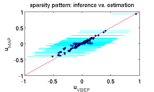
The following scatter plot illustrates the differences between the estimates $\hat{\mathbf{u}}_{MAP}$ and $\hat{\mathbf{u}}_{VB/EP}$ while offering similar predictive performance (16% error). It clearly shows that far more components of $\hat{\mathbf{u}}_{MAP}$ are zero. That means that the MAP estimator puts much more emphasis on driving entries to zero which effectively prunes out features from the model. A posterior mean estimate $\hat{\mathbf{u}}_{VB/EP}$ is far less rigorous. The rationale is that from finite data it is statistically hard to confidently rule out some parts of the model; here the posterior standard deviation (shown in cyan) provides a natural measure of uncertainty.
If a camera is moved while a picture is taken, the resulting image is blurry. If the motion is parallel to the image plane, the measured image $\mathbf{y}\in\mathbb{R}^n$ can be modeled as a noisy convolution of the sharp image $\mathbf{u}\in\mathbb{R}^n$ with a blurring filter/kernel $\mathbf{f}\in\mathbb{R}^f$ as expressed by
\[
\mathbf{y}=\mathbf{f}\star\mathbf{u}+\mathbf{\varepsilon}=\mathbf{X}_{\mathbf{f}}\mathbf{u}+\mathbf{\varepsilon},
\]
where $\star$ denotes the convolution operator which can equivalently be represented by a convolution matrix $\mathbf{X}_{\mathbf{f}}$. We assume Gaussian noise $\mathbf{\varepsilon}\sim\mathcal{N}(\mathbf{0},\sigma^2\mathbf{I})$, $\sigma^2=10^{-5}$.
The model is completed by prior knowledge on the distribution of filter responses of natural images. Multi-scale derivatives as computed by the (orthnormal) wavelet transform matrix $\mathbf{W}$ and the finite difference matrix $\mathbf{D}$ can be combined into a sparsity transform matrix $\mathbf{B}$ whose responses $\mathbf{s}=\mathbf{B}\mathbf{u}$ follow a sparse distribution that is peaked around zero and has heavy tails. The glm-ie toolbox allows the specification of such matrices by a single line of code
W = matWav(su); D = matFD2(su); B = [W; D];where su denotes the size of the image. In the following, we use Laplace potentials $\mathcal{T}_j(s_j)=\exp(-\tau|s_j|)$ where we fix the scale to $\tau=15$.
Estimation
We demonstrate estimation in deblur_estimation.m where we use the convolution matrix $\mathbf{X}_\mathbf{f}$ instantiated by
X = matConv2(f, su, 'circ');We can use non-convex penalty functions like
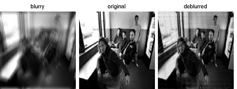
dof = 2; pen = @(s) penLogSmooth(s,dof);to enforce even more sparsity as the Laplace potential or equivalently the penAbs penalty. Note that, the penLogSmooth penalty $\rho(s_j)=\ln(s^2+\epsilon)$ corresponds to the negative log of the Student's t potential. The optimisation problem -- even though non-convex -- can efficiently be solved by LBFGSB or any other solver. For the special case of plsLBFGS, we can enforce nonnegativity $\mathbf{u}\ge\mathbf{0}$ be activating the following flag:
opt.LBFGSnonneg = 1;The figure depicts the original image $\mathbf{u}$ from which the blurry image $\mathbf{y}$ was generated and the reconstructed sharp image $\hat{\mathbf{u}}_{MAP}$ as found be penalised least squares estimation.
Inference
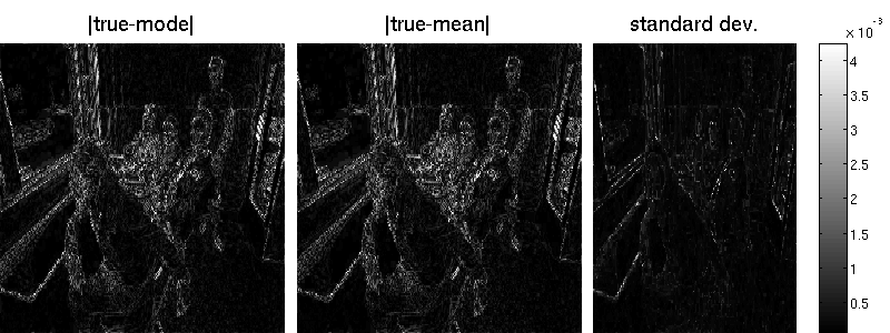
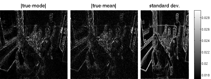
As in the other examples, we can go further and not only find the point of highest posterior density $\hat{\mathbf{u}}_{MAP}$ but to compute a Gaussian approximation to the posterior distribution that allows to quantify the uncertainty in our model. The script deblur_inference.m does exactly this.
Since the marginal variances $\mathbf{z}=\text{dg}(\mathbf{B}\mathbf{A}^{-1}\mathbf{B}^{\top})$ cannot be efficiently computed exactly (due to the $\mathcal{O}(n^3)$ matrix operation, where $n$ is the number of image pixels), we have to resort to an approximation. We use the Lanczos procedure to obtain an estimate $\mathbf{0}\le\hat{\mathbf{z}}_k\le\mathbf{z}$. For $k=n$, the estimate is exact but that is computationally prohibitive for images of realistic size. We can set $k=170$ by
opts.outerVarOpts.MVM = 170;which is much smaller than $n=54910$ in our example.
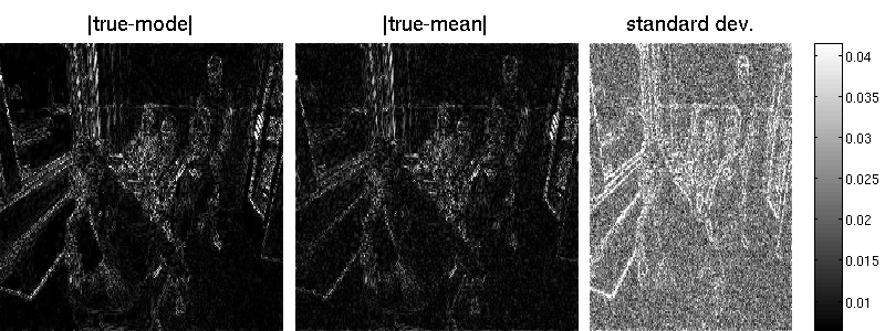
  opts.outerMethod = 'lanczos';       % Lancos
  opts.outerMethod = 'sample';        % Monte Carlo
  opts.outerMethod = 'factorial';     % factorial posterior approximation (MF)
In case, we choose sampling, we can set the number of preconditioned conjugate gradient steps and the number of samples by:
opts.outerVarOpts = struct('NSamples',20,'Ncg',20);
In estimation, we used a wavelet and a finite difference matrix for $\mathbf{B}$; for inference, we only use total variation since the factorial approximation cannot be computed efficiently for the wavelet matrix:
B = matFD2(su);Note that the marginal standard deviations by Lanczos are one magnitude smaller (but also less noisy) than those obtained by sampling. Also the reconstruction error is better for the randomized approach. Note that MAP estimation yields an error of 7.34 in our example (an additional wavelet matrix improves the result, though). Result obtained by Lanzos (error is 7.29):
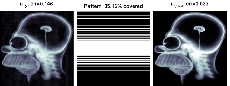
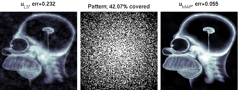
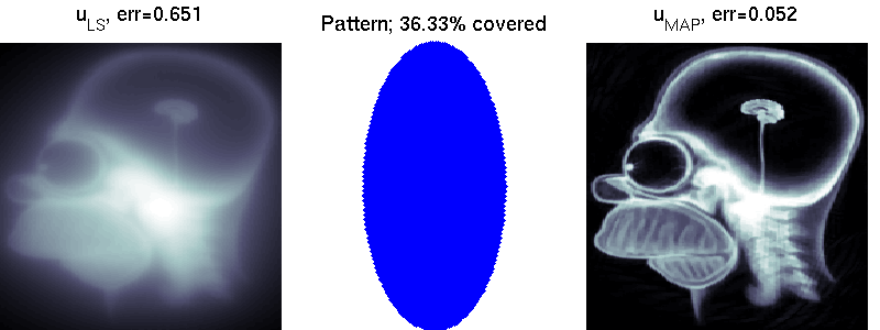
  type_str = {'line', 'mask', 'spiral'};
  type = 2;
The measurement matrices themselves are generated by one of the following three lines of code.
  X = matFFT2line(size(utrue),id,complex,mfull);
  X = matFFTNmask(mask,complex,mfull);
  X = matFFT2nu(size(utrue),k,complex);
Another subtlety comes from the fact that all PLS solvers of the glm-ie toolbox treat real variables only. For that reason, we embed the original complex variable $\mathbf{u}\in\mathbb{C}^n$ into $\mathbb{R}^{2n}$ and solve the corresponding real optimisation problem. The two auxiliary routines mat/re2cx.m and mat/cx2re.m can be used to switch between the two. Also the matrix class mat/@mat and all derived classes mat/@mat* have a mechanism to deal with real and complex vectors: the variable complex specifies whether the matrix $\mathbf{X}\in\mathbb{C}^{m \times n}$ acts as a linear operator $\mathbb{C}^n\rightarrow\mathbb{C}^m$, $\mathbb{R}^{2n}\rightarrow\mathbb{R}^{2m}$ or hybrids thereof.
Estimation
We compare two solvers on the task of undersampled reconstruction of a famous MR image from roughly $40$ percent of the measurements. We can see that simple least squares estimation produces much worse results than PLS estimation.
mri_estimation.m
Several colleagues have helped to improve this software. Some of these are: George Papandreou, Matthias Seeger, Alexander Loktyushin and Michael Hirsch.